The,Different,Distribution,of,Gaussian,Components,between,Mainpulse,and,Interpulse,in,Pulsar,Radio,Profiles

HAN Xiao-hong YUEN Rai

(1 Xinjiang Astronomical Observatory,Chinese Academy of Sciences,Urumqi 830011)

(2 Key Laboratory of Radio Astronomy,Chinese Academy of Sciences,Nanjing 210023)

(3 School of Physics,University of Sydney,Sydney NSW 2006)

ABSTRACT The arrangement of Gaussian emission components along a trajectory traced by a visible point moving at non-uniform speed as the pulsar rotates is investigated.By assuming emission locations confined to spots that arranged evenly around the magnetic axis,a Gaussian emission component corresponds to a cut of an emission spot by the trajectory.The distribution of the emission spots,and hence the Gaussian components,are uneven along the trajectory,being highest around the nearest approach of the magnetic axis to the line of sight,and dependent on two angles of a pulsar:the viewing angle,between the rotation axis and the line of sight,and the obliquity angle,between the magnetic and rotation axes.Observed multiple Gaussian components in a profile then corresponds to several emission spots locating on the trajectory within a specific range of pulsar phase.Demonstration is given to show that the number and distribution of the Gaussian components are different between ranges around the near and far sides of pulsar rotation,corresponding to the mainpulse and interpulse,respectively.The total number of emission spots on a trajectory may be different from that around the magnetic axis,and ignoring the motion of the visible point can lead to significant discrepancy in the predicted number of emission spots.The shape and number of the Gaussian components for fitting a profile may be different from that of the actual components that compose the profile.As an example,the model is applied to the emission arrangement in PSR B0826–34 by assuming the emission comes from a single pole.

Key words radiation mechanisms:non-thermal,pulsars:general,methods:analytical

Investigation of pulsar average radio profiles reveals that they come with vastly different shapes implying that each possesses unique emission arrangement whose details can be obtained by studying the profile characteristics[1–5].An important approach for the latter is to consider each individual profile as a superposition of several emission components of Gaussian shape[6–8].By using a fitting procedure for the set of parameters that minimizes the residuals between the observed profile and the Gaussian components,important details on the geometric arrangements of the emitting structures and the related radio radiation mechanism in the pulsar can be analyzed[1–3,8–14].In principle,the technique is applicable to pulsar profiles of any complexity.Applying to interpulses,second identifiable emission appears roughly at half of a pulsar rotation,the method shows that the number and shape of the fitting emission components are sometimes different from that of the mainpulses.The goal of this paper is to examine the arrangement of Gaussian components at different pulsar phases,and how they relate to the viewing geometry of a pulsar,in particular the viewing angle,ζ,between the rotation axis and the line of sight,and the obliquity angle,α,between the magnetic and the rotation axes.

Arrangement of the Gaussian emission components in a profile usually involves making assumptions for the viewing geometry of the pulsar and the underlying emitting patterns,such as in terms of emission from discrete regions[1–3,12–13].A widely accepted emission model assumes that the emission regions are confined into several isolated and discrete circular sub-beams located on a carousel rotating around the magnetic axis[15–22].In this carousel model,the sub-beams flow around the magnetic axis relative to the surface of the star through the line of sight.A description for the distribution of sub-beams in azimuthal direction around the magnetic axis is attributed to a standing wave at a specific spherical harmonic.The standing wave is determined by an instability in the magnetosphere resulting in a periodic pattern of overdense(sub-beams)and underdense regions of plasma,forming a structure that varies∝cos(mϕb)[23–24],wheremis the emission region number in integer andϕbis the azimuthal angle around the magnetic axis.A favoured instability is the diocotron instability[25–26],although alternatives have also been proposed[23–24].While the distribution of individualmas functions of height,r,and polar angle,θb,is unclear,we assume that radio emission in this version of carousel model appears to come from discrete regions,corresponding tomregions arranged evenly in azimuth around the magnetic axis.Visibility of emission from the regions can then be established by assuming that visible emission from a source point is directed along the local magnetic field line of dipolar structure and parallel to the line of sight.The source point is located within the polar cap region that is bounded by the last closed field lines.Two angles define the geometry,namelyζandα.An explicit solution for the geometry gives the angular position of the“visible point”as a function of the pulsar phase,ψ.As the pulsar rotates,the visible point moves at non-uniform angular speedωV,and traces out a closed path after one pulsar rotation,from where emission is visible to an observer[27].We refer to an emission region from which emission is visible to an observer as an emission spot.The traditional assumption of a stationary visible point is valid strictly forα=0.

In this paper,we investigate the distribution of the Gaussian emission components at different pulsar phases,and its relationship withζandαbased on a purely geometric model.We discuss the viewing geometry and the emission structure used for this investigation in Section 2.In Section 3,we demonstrate the differences in the number of emission spots for a fixed range of rotational phase along different parts of a trajectory traced by the visible point for differentζ,α,and compare them to the scenario whereωVis ignored.We consider the emission arrangement in PSR B0826–34 incorporating the motion of the visible point as an example.We discuss our results and conclude the paper in Section 4.

In this section,we summarize the viewing geometry and emission structure for observable emission.

2.1 Geometry for visible pulsar emission

We assume Cartesian coordinates in which the observer and magnetic frames are represented byandwithandalong the rotation and magnetic axes of a pulsar,respectively,whereω⋆is the spin frequency of the star and the subscript b represents quantities in the magnetic frame.The respective unit vectors in spherical coordinatesandare related by the transformation matrices given in the Appendix4.In the magnetic frame,the equation for a dipolar field line originating from an azimuthal position,ϕb,on the star’s surface is defined byr=r0sin2θbwherer0is the field line constant.

We describe pulsar visibility based on an idealized model in which radiation originates from the source point that locates only within the open-field region[28–29],and the radiation is directed tangentially to the local dipolar magnetic field line[30]and parallel to the line-of-sight direction[27].Designating the polar coordinates of a visible emission in the observer’s and magnetic frames by(θV,ϕV)and(θbV,ϕbV),respectively,a visible point can be defined in the observer’s frame byθ=θV(ζ,α;ψ)andϕ=ϕV(ζ,α;ψ)or by(θbV,ϕbV)in spherical polar coordinates.The visible point in the magnetic frame is given by[27,31]

where cosθc=cosαcosζ+sinαsinζcosψ,andψis measured from the plane whereθcis minimum,orθc=β=ζ−α,withβbeing the impact parameter.For givenζandα,the visible point traces out a closed path on a sphere of radius,r,in the magnetosphere after one pulsar rotation,which we refer to as the trajectory of the visible point.The geometry identifies the center of the pulse profile at the near side to the observer atψ=0 where the rotation axis,magnetic axis and the line of sight are coplanar,andθc=β.We also choose the zeros of all the three azimuthal angles to coincide atϕb=ϕ=ψ=0.Assuming that emission comes only from open-field regions restricts the radiation source be located at heights greater than a height,rV,given by[27]

whereθbLis the polar angle of the point on the last closed field line atϕbV,andθLis the angle measured from the rotation axis to the point where the last closed field line is tangent to the light cylinder.Here,rL=c/ω⋆is the light-cylinder radius andcis the light speed.The minimum and maximum ofrVoccur atψ=0 and 180◦,respectively,in our model.The derivation of Equation(2)is based on the last closed field lines,which are determined by the condition that the field lines are tangent to the light cylinder,and the trajectory of the visible point is tangent to the locus of the last closed field lines[27].Therefore,Equation(2)defines the minimum heights along the trajectory from which emission is detectable.Emission occurring on the last closed field line is visible only fromr=rV.Open field lines satisfyr0>rL,and emission is visible from such field lines only forr>rV.It implies that the minimum height for visible emission from an open-field region isr=rV,which is on the boundary of the region(cf.Section 2.3).The height of a point from which emission is visible is larger thanrVfor field lines located closer to the magnetic axis.

An oblique rotator results in variations in the instantaneous angular velocity of the visible point,ωV,along the trajectory of the visible point given by[27]

whereω⋆=dψ/dt,andωVθandωVϕare two components along the polar and azimuthal directions,respectively.The visible point sub-rotates and reaches the lowest speed when the magnetic axis is on the near side of the pulsar aroundψ=0,but large for a small range aroundψ=180◦,where the emission point super-rotates and reaches the maximum speed when the magnetic axis is on the far side of the pulsar atψ=180◦.The average angular speed over one pulsar rotation is〈ωV(ψ)〉=ω⋆.

2.2 The emission structure

The complicated shape of an average profile in radio pulsars is interpreted as being composed of multiple Gaussian components emitting from discrete locations[6–7].A purely magnetospheric interpretation for the discrete emission locations involves a standing wave structure at a specific spherical harmonic resulting in a distribution that varies∝cos(mϕb)around the magnetic axis[23–24].A periodic pattern ofmenhanced emission regions is formed evenly in azimuth around the magnetic axis,and radio emission from such arrangement appears to come from discrete regions.The configuration of themregions inθbandris uncertain.Here we assume that themregions are arranged in pattern independent of polar angle so that each forms a radial spoke when projected onto a surface of constantr.Furthermore,these spokes are assumed locally independent of height,r.A visible enhanced emission region corresponds to the trajectory of the visible point crossing a spoke,which we refer to as an emission spot.

2.3 Range of visible emission

The visibility of emission requires that(i)an emission point inside an emission spot and both must lie on the trajectory of the visible point,and(ii)the trajectory must lie partly(or entirely)inside an open-field region.The latter introduces a dependence onrfor each open-field line withr=rVcorresponding to the emission point on the last closed field line.The open-field region has a boundary that is fixed relative to the magnetic axis,so that it rotates with the star.The size of the region enclosed by this boundary increases withr,such that it defines the polar cap at the stellar surface,wherer=r⋆,and it extends to all angles forrrL.The pulse-width may be interpreted in terms of the range ofψon the trajectory that lies inside an open-field region and bounded by the points of intersection between the trajectory and the boundary of the open-field region,with the specific value of the fiducial point,ψ0,dependent on the pulsar model.Within the pulse-width,the visible point moves along the trajectory with length that is dependent onr−rV>0,with the pulse-width proportional tor−rV.

Fig.1 shows the trajectory of the visible point(solid black)forζ=10◦andα=20◦,together with three open-field regions with boundaries denoting equal height at 1.4×10−2rL(dotted gray),

7×10−2rL(dot-dashed gray)and 0.14rL(solid gray).The coordinates of a point(xb,yb)in the plot is the Cartesian representation for the coordinate pair(θb,ϕb),and hence the magnetic axis is located at the origin.The relations between the two coordinates are such that a line connecting the origin to the point has length defined byθb,and the angle between the positivexb-axis and the line has range given byϕb.Note that the trajectory does not enclose the magnetic axis.Here,we consider two scenarios.In scenario(i),the motion of the visible point is nonzero,which indicates that the location of visible emission is given by Equation(1).As discussed in Section 2.1,ωVvaries as a function ofψ,whereωV<ω⋆aroundψ=0,and the visible point moves in the direction of pulsar rotation[27].Scenario(ii)ignores the motion of the visible point.This corresponds to visible emission originating from a point where emission is parallel to the line(the line of sight in this case)that passes through the center of the star.As the pulsar rotates,the line remains fixed such that the visible point is stationary in the observer’s frame and the open-field region moves across the visible point at a constant rate atω⋆.Consider first the scenario(i),which is represented by the trajectory in solid black.Emission is visible from heightronly when the trajectory lies within the boundary of an open-field region,and the edges of the pulse window are defined byψwhen the trajectory cuts the boundary.A more restrictive assumption relates to emission occurring only on the last closed field line,and the emission can be seen from only one point of heightr=rV.This is indicated by the inner open-field region,bounded by the curve in dotted gray,with which the trajectory touches its boundary at one point where emission is detectable from that point only.For the open-field region bounded by the curve in dot-dashed gray,the trajectory cuts it from pointsAtoBbetween which the trajectory lies inside.Their longitudinal phases areψA=−90◦andψB=90◦giving the range of observable emission ∆ψ=ψB−ψA=180◦.A special case is shown with the outer open-field region,bounded by the curve in solid gray,where the trajectory is enclosed entirely in the region.This implies that emission from locations that coincide with any points on the trajectory is observable giving a pulse-width that spans over the entire pulsar rotation.For scenario(ii),the location of the visible point is fixed at a polar angleθ=θVatψ=0 in the observer’s frame and the open-field region moves across it as the pulsar rotates.Transforming to the magnetic frame using the equations in the Appendix4 gives a path that is different from the trajectory of the visible point,as shown by the dotted black curve.The discrepancies are due to omission of the changing location of the visible point associated with the variation ofωVas the pulsar rotates.Here,the path intersects the inner region at the same point as the trajectory of the visible point.For the open-field region in the middle,it intersects the boundary differently at locationsA′andB′whereψA′=−50◦andψB′=50◦giving a pulse-width that is almost 45%narrower.The different path means that emission originates from different set of open-field lines withr0>rL,andr=1.4×10−2r0atψ=0.Instead of enclosed by the outer region,as with the trajectory of the visible point,the path intersects the region at pointsCandD,withψC=−75◦andψD=75◦.This implies that emission is observable only at locations where the path lies inside the region and betweenψCandψD.The required height at the boundary of an open-field region to enclose the entire path is now 0.32rL,which is higher by more than twice of the value when the motion of the visible point is included.

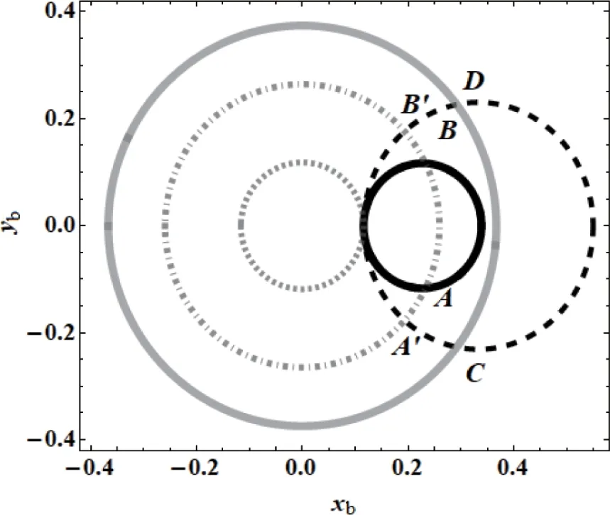
Fig.1 Simulations for different pulse-widths based on three open-field regions with boundaries at increasing height from inner at 1.4×10−2 r L(dotted gray)to outer at 0.14r L(solid gray)for a trajectory of the visible point(solid black)using ζ=10◦andα=20◦.The magnetic pole is located at the origin.See text for explanation of the points A,B,A′,B′,C and D.Also shown is another path(dotted black)for visible emission where the motion of the visible point is ignored.Note that x b and y b are normalized.

In this section,we show that the distribution of emission spots,corresponding to the distribution of the Gaussian components,along the trajectory of the visible point is uneven and generally different from that around the magnetic axis.We also examine the significance of ignoringωV.

3.1 Along the trajectory of the visible point

We simulate four trajectories of the visible point in theψ-ϕbplane that is constructed similar to the equirectangular projection for mapping a globe.In this representation,the distances along the line of longitudes are conserved such that the magnetic pole is a vertical line alongψ=0 as shown in Fig.2,which shows the variations ofϕbValong the trajectory of the visible point as a function ofψfor different values of{ζ,α}.For better illustration,20 radial spokes(gray horizontal bands)are assumed evenly in azimuth around the magnetic axis giving horizontal rows of spoke with the two spokes centered atϕb=−180◦andϕb=180◦coinciding with each other.Pulsar rotation is counterclockwise when looking directly down the rotation axis where the direction of rotation is pointing upward.As the pulsar rotates,the visible point moves starting fromψ=−180◦and advances to more positiveψtracing out a trajectory that ends atψ=180◦after one complete pulsar rotation.According to Equation(1),a corresponding traversal inϕbthat covers from−180◦to 180◦signifies a complete revolution around the magnetic axis.The evolution ofϕbis different for different trajectories as shown in Fig.2.For a trajectory withβ>0,such as the one in solid blue,the variation inϕbfirst decreases negatively towards and approaches−180◦asψincreases,and reachesϕb=180◦atψ=0,where the visible point is located between the magnetic axis and the equator.It then decreases asψincreases and returns toϕb=0 forming a complete rotation around the magnetic axis.For a trajectory withβ<0,as the one in solid black,the variation ofϕbis also increasing negatively to a minimum(>−180◦),then decreases and reachesϕb=0 atψ=0,where the visible point is located between the magnetic and rotation axes.It then increases again positively reaching a maximum(<180◦),then decreases and returns toϕb=0.Variation inϕbValong a trajectory as the pulsar rotates results in cutting spokes in the process with the number that is dependent onζ,α.Fig.2 shows that not all trajectories enclose the magnetic axis.A complete revolution around the magnetic axis occurs only for the trajectories in blue and brown,both with positiveβ,whereas a partial coverage is seen for trajectories in black and green,whoseβvalues are negative.

Fig.2 Variations of ϕb along the trajectory of the visible point as a function of ψ for{ζ,α}={30◦,15◦}(solid blue),{10◦,20◦}(solid black),{40◦,30◦}(solid brown)and{40◦,43◦}(solid green).A stationary 20-spoke structure is shown for−180◦≤ϕb≤180◦with each spoke assumed of 9◦in width.Radial spokes at the sameϕb line up and appear as a single spoke(gray horizontal band)in theψ-ϕb plane.Evolution of a trajectory is toward more positive ψ.Trajectories are not straight lines indicating non-uniform variation of ϕbV resulting in uneven distribution of emission spots on a trajectory.Also shown are two pulse windows,each of width 80◦,centered at ψ=0 and bounded by two gray vertical lines,and at ψ=180◦,bounded by two vertical dashed lines,within which each trajectory intersects different number of spokes.The dotted curves represent paths that traced by a visible point using the sameζ,α of the corresponding color but with ωV omitted.

Auniform distribution of radial spokes around the magnetic axis does not imply evenly distributed emission spots along the trajectory of the visible point.For nonzeroζ,α,variation ofϕbValong a trajectory is large for ranges aroundψ=0 then reduces towardψ=±180◦.A special case relates toζ=0(not shown)whereϕbVis a constant resulting in a horizontal line.A larger change inϕbVfor a given change inψmeans that more emission spots are visible as the trajectory cuts more spokes.Considering−40◦≤ψ≤40◦(between two vertical solid gray lines)in Fig.2,the corresponding coverage of∆ϕb=∆ϕbVis 131◦(solid blue),56◦(solid black),168◦(solid brown)and 137◦(solid green)cutting 7,3,9 and 7 entire spokes,respectively,where the last trajectory also cuts a fraction of two spokes centered atϕb=±72◦.However,the corresponding changes inϕbfor the same amount of changes inψat aroundψ=±180◦are smaller.

A different view on the uneven number of observable emission spots for a given range ofψalong a trajectory of the visible point is through the consideration of the change ofϕbVin terms ofψ.Fig.3 shows the variation in ∆ϕbV/∆ψas a function ofψfor the sameζandαcombinations used in Fig.2.A negative value indicates that a trajectory is advancing in the oppositeϕbdirection,as seen by the case with the trajectories in black and green for|ψ|≿50◦.A special case is shown forζ=0(red)where theϕbVis a constant resulting in a horizontal line at ∆ϕbV/∆ψ=0.In general,ζ̸=0 and the curves peak at aroundψ=0,with the change in ∆ϕbV/∆ψbecoming steeper asβlowers for a givenα.Cutting of a radial spoke by the trajectory is signified by the traversal of the latter through all or part of the spoke inϕb,and more spokes are cut for a broader coverage inϕb.Therefore,∆ϕV/∆ψmay be treated as the density of spokes cutting by a trajectory of givenζ,α.The density increases asψapproaches zero(more spokes are cut)and decreases as|ψ|increases.Variations in the density then imply uneven distribution of emission spots,corresponding to different numbers of Gaussian components,along the trajectory with the emission spots appearing to bunch up more aroundψ=0 where the density is highest.

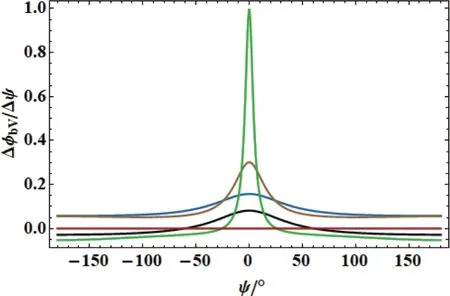
Fig.3 Normalized ∆ϕbV/∆ψas a function of ψ indicating changes in the density of observable emission spots as a function of ψalong the trajectory of the visible point for the same four combinations of ζ,αinFig.2.The red horizontal line indicates ζ=0,α=60◦.Note that absolute values are taken for the blue and brown curves.

3.2 Distribution around the far side of rotation

Figs.2 and 3 suggest that an unequal amount of emission spots is cut at nearψ=180◦as compared to that aroundψ=0.The number of radial spokes cut by each trajectory for the same∆ψ(between the two vertical dotted lines)centered atψ=180◦is 3(solid blue),1(solid black),3(solid brown)and 3(solid green)as shown in Fig.2,which is less than that cut at aroundψ=0 as each covers a smaller range ofϕb.For emission coming from a single magnetic pole and a profile with the fiducial point located atψ=0,the number of constituting emission components for a profile centered atψ=0 is different from that atψ=180◦for identical ∆ψ,with the former being larger.It follows that,if each emission spot radiates equally,the flux density of a profile is weaker aroundψ=180◦as it comprises lesser emission spots,corresponding to fewer Gaussian components.

3.3 Total observable emission spots

An emission is detectable only if the corresponding emission spot lies on the trajectory of the visible point.It follows that the estimation of the total number of emission spots is along the trajectory of the visible point,which may or may not enclose the magnetic axis.This yields a number that may be different from that located around the magnetic axis.A prominent example is that shown with the trajectory in black in Fig.2 where the observed number of emission spots are different from the assumedm=20.For the cases considered in Fig.2,only the trajectories in solid blue and solid brown,both with positiveβ,give a prediction of 20 emission spots,whereas the others give a lower values at 6(solid black)and 16(solid green).

3.4 Omission of ωV

The significance of the motion of the visible point is revealed by considering another scenario in which the visible point is assumed stationary,as discussed in Section 2.3.The resulting path traced by the visible point for each of the combinations ofζ,αin Fig.2 is shown in dotted lines of the corresponding color.The two scenarios coincide at only two points atψ=0 and 180◦,and the greatest discrepancies occur aroundψ=0 where the line of sight is closest to the magnetic axis in the model.The range ofϕbcovered by each path is also different with ∆ϕb=148◦(dotted blue),83◦(dotted black),181◦(dotted brown)and 142◦(dotted green)for|ψ|≤40◦.The number of predicted emission components for the corresponding path are 9,5,11 and 9 for|ψ|≤40◦and 3 for all trajectories for|ψ|≥140◦.While the total number of predicted emission spots for the trajectories in blue,brown and green remains the same,it is different for the trajectory in black with a total of 10 emission spots predicted.The deviations are expected to be more significant when the constraints on the height of an open-field region is imposed as shown in Fig.1.This is because the path that traverses an open-field region of a particular height is longer whenωVis omitted implying that more emission spots are cut.However,∆ψactually diminishes meaning that the visible point spends a shorter time in an open-field region.

3.5 Profile with small∆ ψandβ

The assumption that pulsar radio profiles can be represented by multiple components of Gaussian shape[7–8,32]represents an essential technique for studying pulsar emission structures and properties.The identification of the constituting components of a profile is achieved by fitting a sum of Gaussian components to the profile of interest.To avoid over-fitting,a measure of some kind is established for comparison of the fitted and observed profiles and one will stop adding components to the fitting once the value given by the measure is below a certain threshold[6].As the amount of fitting components is different for different pulsars[6],an important aspect of such analysis relates to the questions of the“true”number of the“real”components.This is due to the fact that the obliquity angles of many pulsars are unknown and hence it lacks a method to estimate the true number of the constituting Gaussian components.Failure of such decomposition is a known effect if the observed profile is not well resolved resulting in the fitting being not unique or even correct.This introduces bias in subsequent analysis for the emission properties of the pulsar.

In general,the number of emission spots cut by a trajectory of the visible point is dependent on the viewing geometry such that the former increases as|β|decreases for a fixed∆ψ.It is consider a scenario whereα=30◦andβ=0.5◦,which gives nine emission spots for ∆ψ=10◦.Next,we construct the Gaussian component for each of the emission spot by randomly1We explored different configurations,both random and organized,and obtained similar results.generating the amplitude,J,between 0.1 and 1,pulse-width,σ,based on one-fifth to full size of a radial spoke in degrees,and the position of peak phase,ψp,that fits within ∆ψ=10◦.The organization of the components is such thatσdecreases as the peak phase(|ψp|)increases toward the two boundaries of the profile.The profile is then given by the sum of all the components with the intensity varies as[6–7,11]

whereIis the intensity of the profile as a function ofψ,isignifies theith Gaussian component,andNis the total number of components,which is nine in this case.Table 1 lists the parameters required for simulating and fitting the same profile.The parameters for each Gaussian component are given in the upper panel of Table 1,and their shapes and the resulting profile are shown in Fig.4.Note that random noise has been added to the resulting profile to mimic real observation.The simulated profile in Fig.4 would represent an observed profile.Assuming no knowledge of the original components,we try to fit the same profile(with noise)using different sets of Gaussians,each containing different number of components from one to eight.Then,the observed profile is simulated for 100 times,each with different random noise,and an average value for the residual sum of squares(RSS)from the fitting is calculated for each set.Fig.5 shows the fitting for the original profile shown in Fig.4.The least number of Gaussian components that gives the best fitted profile is shown in gray and red,respectively,in Fig.5,with the latter overlaying with the original profile(black).The parameters are given in the lower panel of Table 1.From Fig.5,the residuals for the difference between the fitted and simulated profiles exhibit random scattering around zero with the mean and maximum values given by−8×10−4and 0.07 in intensity,respectively.The average RSS is about 5.8.As a comparison,using the original nine Gaussian components(in Fig.4)for the fitting also gives RSS of about 5.8 in average.This suggests that the fitting using the four Gaussian components is reasonably well.However,it is clear from Fig.5 that the number of Gaussian components needed to fit the profile,NF,is different from the actual number of components,NC,that composes it.In general,we find thatNF≤NC.

Fig.4 Simulation of the profile(black)using nine Gaussian components(gray)based on the parameters in Table 1 forβ=0.5◦andα=30◦within a pulse-width of 10◦centered atψ=0.Random noise has been added to the resulting profile.

3.6 An example case:PSR B0826–34

Emission from this pulsar can be detected from most of the pulsar rotation resulting in a broad profile[33–34].Esamdin et al.[34]divided the profile in strong-emission mode into four distinct regions based on the emission and subpulse properties,with emission mostly detected in regions I and III.The shapes of the profile from these two regions both imply composition of more than one emission component,with region III displaying five discernible components and a similar number of components but more bunched up in region I.Furthermore,the range of detectable emission is also different for the two regions with region I being narrower giving a slightly higher density in emission component.Based on the differences in the variations of the subpulse spacings between the first and second half of the profile,the authors were able to estimate an obliquity angle of 0.5◦for this pulsar suggesting that both emission comes from a single magnetic pole[34].

Fig.5 Fitting for the original profile in Fig.4 by using fewer Gaussian components(gray).The original and fitted profiles are indicated in black and red,respectively.

We simulate the trajectory of the visible point incorporating the motion of the visible point using the predictedα=0.5◦and an assumedβ=2.3◦.An observed higher density of emission component in region I implies that the corresponding part of the trajectory lies in the range of pulsar phase aroundψ=0 in our model.With the reported pulse windows of sizes 94◦and 143◦for regions I and III[34],respectively,we divided the trajectory of the visible point into four parts,such that the range betweenψ=±47◦,centered atψ=0,corresponds to region I and fromψ=88.5◦to−128.5◦corresponds to region III.A total number of 14 radial spokes is assumed evenly located around the magnetic axis.Our model predicts an openfield region at height≿13r⋆,wherer⋆=10 km is the stellar radius,for observable emission to come from the trajectory of the visible point due only to a single magnetic pole.The trajectory revolves around the magnetic axis and traversesϕbfrom−125◦to 125◦in total of ∆ϕb=110◦for region I,and from 81◦to−44◦in total of ∆ϕb=125◦for region III.A non-uniform spoke density along the trajectory is determined with the highest density occurring in region I and lowest in region III giving an estimation of 5 emission spots in both regions consistent with observation.To simulate the profile with drift phases adjusted,as shown in Fig.4 by Esamdin et al.[34],we assume thatσis given by half the spoke size for all Gaussian components,which isσ=6.4◦for 14 spokes around the magnetic axis.The peaks for the components as given by our model are located atψ=−43.4◦,−21.5◦,0,21.5◦,43.4◦for region I,and atψ=92.8◦,120.7◦,149.8◦,180◦,−149.8◦for region III.We also assume that the amplitude(J)for the emission spots in region I is twice as that in region III.Fig.6 shows the profiles in regions I and III coinciding with the reported longitudinal phases.The simulation reproduces several basic features of the observed profile.Firstly,five pulse components are obtained for the two regions,with the separation between components being wider in region III.The pulse-width measured at 10%of the full intensity is also wider in region III than that in region I at 145◦and 115◦,respectively.In addition,a drop in intensity is seen between any two consecutive pulse components,with the ratio of drop(relative to the average peak intensity of the two immediate adjacent pulse components)being larger in region III,consistent with observation.The same is seen regardless ofJchosen in the two regions.Furthermore,the amount of the intensity drop varies across the simulated profiles.Asψincreases,the amount of drop exhibits decreasing followed by increasing in region I,whereas it is varying in region III.Both are consistent with the observation.Our simulation also indicates variations in the emission spot separation(P2)across the profile with an average of 22◦in region I,consistent with observation,and slightly higher at 29◦in region III.

Table 1 Parameters of the Gaussian components for simulation and fitting the same profile are shown in the upper and lower panels,respectively.The numbers are rounded to two decimal places

Fig.6 Simulations for the profile(drift phases adjusted)for regions I(left)and III(right)

We have investigated the distribution of emission components based on a purely geometric model in which detectable emission at a particularψcomes from a visible point where emission is tangent to the dipolar field line and directed parallel to the line of sight direction.The visible point moves at non-uniform speed as the pulsar rotates tracing out a trajectory that may or may not enclose the magnetic axis.By assuming an emitting structure in which emission is confined to spots that are arranged uniformly around the magnetic axis,a Gaussian emission component corresponds to emission from an emission spot that lies on the trajectory of the visible point.In this model,the distribution of emission spots on the trajectory of the visible point is uneven being highest aroundψ=0 and lowest aroundψ=180◦.We show that the viewing and obliquity angles of a pulsar can affect the amount of emission spots determined along a trajectory,which may be different from the total number of emission spots around the magnetic axis.We compare our model to those withωVignored and find that the predicted number of emission spots can be different both for a given range of ∆ψnearψ=0 and along the whole trajectory.We consider PSR B0826–34 as an example and show that,by treating emission from a single pole andm=14,our model can account for the observed number of emission components,and some related characteristics,in the two emission regions corresponding to the mainpulse and interpulse.

Our model is consistent with the fact that pulsar average radio profiles are generally composed of multiple emission components.This is shown in Fig.2 where each of the trajectories cuts more than one emission spot regardless of the sign ofβ.Since the density of emission spots changes as the trajectory traverses longitudinal phases of different ∆ϕbV/∆ψ,intersection of multiple emission spots requires that the trajectory is steep aroundψ=0 implying smallβ.This is consistent with most pulsars whoseβ<10◦[1]and a typical duty cycle of 0.1 resulting in the trajectory that covers broad ∆ϕbVand hence cutting multiple emission spots.For pulsars with smallβand∆ψ,the arrangement of the emission spots is such that they locate closely to each other within a narrow range of pulsar phase resulting in overlapping with neighboring Gaussian components.In this case,modest deviations in the emission properties across the emission spots,due to their locations being at different parts of the carousel layer,may be masked by other components giving an overall simpler profile shape as shown in Fig.4.This leads to deviation in the prediction of the number of emission spots,which compose the profile,from the number of Gaussian components used for fitting the profile.It also implies that the shape of a profile may appear“simple”but the actual amount of composing emission components may be many.

The prediction of a non-uniform distribution of emission spots along the trajectory of the visible point even for a uniform arrangement of emission spots around the magnetic pole has implication on drifting subpulses and the observed drift rate.Drifting subpulses manifest as a systematic flow of subpulses across the pulse window resulting in tracks traced by the drifting subpulses in consecutive pulses.A parameter,known asP2,is used to describe the separation between two consecutive subpulses.In our model,P2corresponds to the time interval that the visible point takes to cut two consecutive emission spots.Another parameter,designated asP3,represents the time for the drift pattern to repeat once,with the drift rate given byP2/P3.Adistinction can be made between the flow of subpulses around the magnetic axis and the observed drifting of subpulses through the line of sight.The former corresponds to movement of the radial spokes in our model around the magnetic pole(along theψ=0 axis)towards either increasing or decreasingϕbdepending on the drift direction.This movement can be steady or varying being a function ofϕb.In either case,a relative motion exists between the visible point and the spokes,with the magnitude changes along the trajectory of the visible point.This relative motion contributes to the observed separation between the emission spots.We consider constant movement of spokes toward more positiveϕband a viewing geometry represented by the trajectory of the visible point in solid green whereψadvances from−180◦to 180◦as the pulsar rotates.The visible point will encounter emission spots moving in opposite direction between|ψ|≿40◦giving a higher relative motion.For|ψ|<40◦,the emission spots appear to move in opposite(same)direction for slower(faster)moving spokes than the visible point with both situations leading to a slower relative motion.It is apparent from Fig.2 that the difference in the measured separation between consecutive emission spots(P2)and the flow rate of the radial spokes around the magnetic axis is dependent onζ,α,with the difference intensifies for increasingly smaller|β|.AssumingP3is constant,the variations inP2imply changes in the drift rate.Therefore,measurement of drifting subpulses is inevitably linked to the emission geometry of the pulsar.

There are obvious limitations in our model.Firstly,we assume circular carousel layers,with uniform arrangement of emission spots on each layer,and concentric at the magnetic axis in a pure dipolar field structure.The resulting emission geometry is self-similar in the sense that the traversal of an emission spot by the trajectory of the visible point is independent ofr.The observed asymmetric separation between the mainpulse and interpulse in PSR B0826–34 implies deviation of the above assumptions.A more accurate model will need to include the distortional effects due to ther−2andr−1terms in the magnetic field equation.In this case,a circular carousel layer is expected to become more distorted as it locates increasingly away from the magnetic axis and the associated distribution of emission spots is unlikely to be uniform anymore but will also be dependent onrandϕb.Secondly,pulsar emission is attributed to highly relativistic particles propagating along magnetic field lines and directed along the velocity of the particles,which is not strictly along the magnetic field line but vastly confined to a narrow forward cone.Furthermore,the cone angle is not zero and the angular difference between the axis of this cone and the field line is proportional to emission height.For a pure dipolar structure,as we assumed in this investigation,which applies only to the lowest order in an expansion inr/rL,these deviations are small and can be included as perturbations.In its present form,our model is incapable of predicting the conical structure and offers no information on the grouping of the emission spots into either inner or outer cones within a profile.

AcknowledgementsWe thank the XAO pulsar group for discussions.We also thank the anonymous referee for useful comments which have improved the presentation of this paper.

Appendix

Transformation matrices

The transformation between the unit vectorsandis given by

where

andRTis the transpose ofR.For transformation between Cartesian to the respective unit vectors in spherical coordinatesand,we have

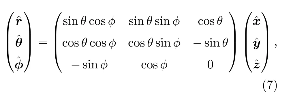
and transforming vectors relative to the magnetic axis involve adding the subscript b to Equation(7).