Measurement,of,T,wave,in,magnetocardiography,using,tunnel,magnetoresistance,sensor

Zhihong Lu(陆知宏) Shuai Ji(纪帅) and Jianzhong Yang(杨建中)

1Department of Precision Instrument,Tsinghua University,Beijing 100084,China

2Beijing Innovation Center for Future Chips,Beijing 100084,China

3State Key Laboratory of Precision Measurement Technology and Instruments,Tsinghua University,Beijing 100084,China

Keywords: magnetocardiography,tunnel magnetoresistance,optically pumped magnetometer,T wave detection

Magnetocardiography (MCG) measures the magnetic field produced by the electrical activity of the human heart near the torso.[1]MCG is a promising technique for clinical application since it provides more accurate information for cardiac diagnosis than electrocardiogram (ECG).[2]The major clinical applications of MCG include myocardial ischemia detection,arrhythmogenic risk assessment,and fetal MCG.[3]

Accurate measurement of MCG is a prerequisite for its application.Typically, the maximum amplitude of MCG signals is about 100 pT.Only magnetic sensing techniques with high sensitivity and low noise can detect MCG.A superconducting quantum interference device (SQUID) is generally used for MCG measurement.Nevertheless, SQUID is an expensive and bulky equipment with high running costs due to the use of liquid helium.The optically pumped magnetometer (OPM) has also been widely noticed because of its excellent performance similar to SQUID.Several OPMs capable of MCG measurements have been reported.[4-6]In recent years, tunnel magnetoresistance(TMR)sensors have become a new technique to measure MCG due to their low power consumption and the ability to measure MCG in unshielded environments.[7]The study of Kosuke Fujiwaraet al.achieved the detection of MCG R wave,[8]and the study of Meiling Wanget al.acquired triaxial MCG signals.[9]Real-time measurements of MCG QRS components were also achieved using new low-noise TMR sensors.[10]

The T waves of MCG are the peaks corresponding to ventricular repolarization.[11]Repolarization is an important physiological process in the heart, so the T wave contains essential clinical information.MCG provides betterrecognizable T waves than ECG, which is an important reason why MCG can achieve higher diagnostic sensitivity.[12]The time differences between T wave and P wave,T wave and Q wave are named PT interval[13]and QT interval, respectively.The PT interval provides the information to diagnose ischemic heart disease (IHD).[14]The QT dispersion which measures the difference between the maximum and minimum QT intervals is a crucial MCG feature for arrhythmogenic risk evaluation.[15,16]SQUID,OPM and spin exchange relaxation free(SERF)magnetometers are able to clearly measure the T waves of MCG.[12]However,the T waves of MCG measured by TMR were drowned by noise in most previous study and the accuracy of T waves measured by TMR has not been studied.As a new method, the clinical value of TMR for MCG measurement is profoundly affected by the T wave accuracy.Achieving accurate T wave measurements will allow TMRbased MCG measurements to provide an essential basis for cardiac medical diagnosis.

This study measures MCG by a low-noise TMR sensor,and the T wave is clearly presented after baseline drift suppression and averaging.MCG measured by TMR is compared with the MCG measured by OPM at the same position.This is the first comparison of MCG measured by TMR with MCG measured by the higher precision OPM.[17]The time and amplitude of the T wave are used as parameters for its accuracy and our experiments demonstrate that the TMR can accurately measure the two parameters.

2.1.TMR sensor

TMR consists of magnetic tunnel junctions(MTJs)which are structures stacked by pinned layers,tunnel layers,and free layers.The resistance of MTJ is determined by the difference in magnetization orientation of the pinned layer and the free layer.The greater the difference,the greater the MTJ resistance.The external magnetic field changes the resistance of MTJ by affecting the magnetization orientation of the free layer.

The TMR sensor used in this paper is a push-pull structure consisting of four resistorsR1,R2,R3,andR4.The magnetization orientation of the pinned layers of MTJ in the four resistors is shown in Fig.1(a).TheR1andR4are magnetized in the same direction,whileR2andR3are both in the opposite direction.Thus,the output voltage of TMR can be calculated according to the following equation:

where ΔR1,ΔR2,ΔR3,ΔR4are the absolute resistance change ofR1,R2,R3,andR4under an external magnetic field,respectively.VSis the bias voltage applied to the bridge.

Fig.1.(a) TMR Wheatstone bridge and structure schematic of MTJ components.Four resistors R1, R2, R3, and R4 form the bridge.MTJs in each resistor are stacked by pinned layers, tunnel barriers, and free layers.The direction of the arrow in the pinned layer indicates the magnetization direction.The double arrow in the free layer indicates that its magnetization direction is variable.VS is the bias voltage,while V1 and V2 are the outputs of TMR.(b)A photo of the TMR sensor,the direction of the double arrow is the direction of the sensitive axis.

The size of the integrated TMR sensor is 29.0 mm×11.8 mm×2.5 mm, and the sensitive axis is along the line direction shown in Fig.1(b).The main performance parameters of the TMR sensor are listed in Table 1.The bias voltage applied is 5 V,and the fit range for calculating sensitivity and linearity is-0.3 Gs to 0.3 Gs.The resistance of the TMR sensor is 2057.2 Ω, and the sensitivity is 3.1 µV/nT.The definitions of TMR sensors’ linearity and hysteresis are consistent with the previous study.[9]The linearity and hysteresis of the TMR sensor are 0.7%and 0.14 Gs,respectively.

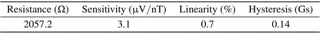
Table 1.Performance parameters of the TMR sensor measured in the range of-0.3 Gs to 0.3 Gs.

2.2.Signal conditioning circuit

The schematic diagram of the signal conditioning circuit of the TMR sensor is shown in Fig.2.The output of the TMR sensor is first amplified 100 times by the instrumentation amplifier AD8429.The DC bias,mainly caused by the asymmetry of the TMR bridge,is then removed by a differential amplifier circuit with gain 5.An adjustable DC voltage in the range of-3 V to 5 V is input atVBias1to offset the DC bias.Next,the signals pass through a second-order low-pass filter with a cut-off frequency of about 150 Hz and gain 25.The low-pass filter will effectively suppress high-frequency noise.Finally,another differential amplifier circuit with gain 18 eliminates the newly introduced DC bias.VBias2is connected to another adjustable DC voltage varying from-3 V to 5 V.

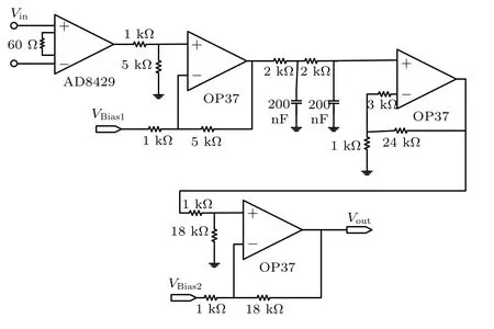
Fig.2.Signal conditioning circuit schematic.

Fig.3.Noise density spectrum of the TMR magnetometer in the magnetically shielded environment.

2.3.MCG measurement

MCG measurement experiments were performed in a large four-layer MSC.The outermost layer of MSC is aluminum alloy, and the inner three layers are permalloy layers.The residual magnetic field in the direction of MCG measurement is less than 5 nT.

The OPM used to measure the MCG is a commercial single-channel OPM produced by QuSpin,Inc.The probe has a reasonably small size of 12.4 mm×16.6 mm×24.4 mm.The typical noise level of this OPM is 10 fT/Hz1/2, which is much smaller than the noise of TMR.The noise performances of the OPM, TMR used in this paper and other MCG measurement methods are listed in Table 2.The performance of OPM reaches the highest echelon.The performance of TMR is relatively low but better than induction coil gradiometers.

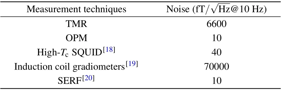
Table 2.Performance comparison of TMR, OPM and several other MCG measurement methods.

The measurement is performed in two steps.The first step is the measurement of MCG by TMR and OPM at different positions.The OPM acquires the reference signal for averaging MCG measured by the TMR.The OPM is 40 mm to the right of the center of the chest.The TMR is 40 mm to the left of the center of the chest and 30 mm downward.A diagram of the experimental setup for the first step is shown in Fig.4(a).The second step is that the OPM measures MCG at the same position as the TMR,as shown in Fig.4(b).The two-step experiment was performed consecutively, with the MCG being measured for approximately 5 min in each step.The sensors’sensitive axis is oriented in the direction of the arrow in Fig.4.

The MCG of a 24-year-old male subject in the supine position was measured.The distance from the center of the TMR sensor and the OPM sensor to the body surface is 2 mm and 8 mm, respectively.The sampling frequency for both TMR and OPM is 1 kHz.

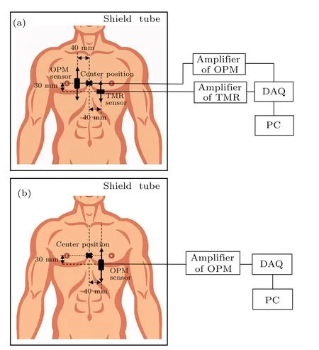
Fig.4.Experimental setup for MCG measurement using TMR and OPM:(a)the first step,(b)the second step.The source of the picture of the human body in the figure is https://www.vcg.com/creative/1142486167.

3.1.Baseline drift removal

The TMR sensor is close to the body and the heart when measuring MCG.Significant baseline drift is mixed in MCG due to respiration, heartbeat, and other disturbances.Lowfrequency drift is processed first.

The empirical mode decomposition (EMD)[21]decomposes a signal into several simple oscillatory modes called intrinsic mode functions (IMFs).To improve the stability of decomposition and the accuracy of the reconstruction, new versions of EMD have been proposed.[22-24]The version of EMD used in this work is the improved complete ensemble empirical mode decomposition with adaptive noise(improved CEEMDAN).[24]

To remove the baseline drift, the original MCG dataxis first decomposed into IMFs and residue, and it can be expressed as

wherediis thei-th IMF,Iis the number of IMFs,andris the residue which can also be regarded as a special IMF.

These IMFs and the original data are shown in Fig.5.The IMFs occupy successive frequency bands.The smaller the order of the IMF,the faster the oscillatory.As a result,the low-frequency baseline drift concentrates in the last few IMFs.The frequency of baseline drift does not exceed the heart rate.In contrast,the frequency components of MCG waves are generally higher than the heart rate.Since the heartbeat also introduces interference, we consider IMFs with oscillation frequencies not exceeding the heart rate as the baseline drift.The baseline drift is then obtained by summing these IMFs.

Fig.5.IMFs of the MCG data measured by TMR after improved CEEMDAN.From top to bottom: MCG raw data and its IMF1-12.

To measure the effect of the improved CEEMDAN on the MCG signal,a simulation experiment is conducted.Synthetic baseline drifts are added to MCG signals and then the noisy MCG signals are processed by the improved CEEMDAN.A low frequency (0.3 Hz) sinusoidal signal is used to simulate the baseline drift.[25]The MCG signal is a synthetic signal,[26]which does not contain noise.Baseline driftu[n] of different amplitudes is added to the MCG signals[n],and the input signal-to-noise ratio(SNR)is used to measure the magnitude of the baseline drift relative to the MCG signal.The input SNR is calculated as

The MCG with additive baseline drift is processed by the improved CEEMDAN and noted asy[n].The output SNR is used to measure the change of the processed signal relative to the original MCG.The output SNR is calculated as

Table 3 shows the output SNR results when the input SNR is from-7 dB to-15 dB.It can be seen that the output SNR has a significant improvement concerning the input SNR, which means that the improved CEEMDAN effectively removes the baseline drift.The output SNR values exceed 8.5 dB at different input SNR, demonstrating that th eimproved CEEMDAN processing does not have a destructive effect on the MCG signal.

Here we return to the MCG signal measured by the TMR sensor.Figure 6 shows the original MCG signal and the baseline drift extracted using the improved CEEMDAN.The baseline drift exactly fits low-frequency oscillations in the raw data and is removed by subtracting it from the original signal.

Table 3.Output SNR of improved CEEMDAN with different amplitude noise inputs.

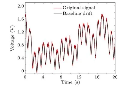
Fig.6.Comparison of the baseline drift extracted by the improved CEEMDAN and original MCG data.

3.2.MCG measured by TMR

Figure 7 shows the MCG signal measured by TMR after removing the baseline drift.Apparent noise can be observed in the MCG signal.The MCG measured by TMR is averaged triggering on the R peak to handle the noise,and the R peak identification is made with the reference MCG signal measured synchronously by OPM.

Fig.7.Real-time MCG measured by TMR after removal of baseline drift and reference MCG measured by OPM.

The single-cycle MCG signals measured by TMR and OPM at the same position are shown in Fig.8.The MCG raw data measured by TMR is shown in Fig.8(a).The noise in MCG raw data is apparent, but waveform features can be observed.Averaging the MCG measured by TMR was performed using the R peak of the synchronous MCG recorded by the OPM to improve the SNR.The average number of MCG measured by TMR is chosen to start from 16 and increased by 16 each time until the noise superimposed on the T wave is no longer significant.The average number of MCG measured by OPM is selected based on the absence of visible power line interference after averaging.Figures 8(b) and 8(c)show the MCG signals when the averaging is performed 16 and 32 times,respectively.Noise decreases significantly in both graphs.The R wave, S wave, and T wave of MCG are clearly visible in Fig.8(c).Figure 8(d) shows the MCG signal averaging 40 times and measured by the OPM at the same position as the TMR.The magnetic field amplitudes related to the R peaks measured by TMR and OPM are approximately 220 pT and 120 pT, respectively.The difference in R peaks amplitude is due to the different distance between the centers of the two sensors and the body surface.The MCG for both measurements shows a T wave at about 0.4 s to 0.5 s.To our best knowledge,this is the first time that the T wave of MCG measured by TMR is compared to another measurement technique.

A comparison of the T wave of MCG measured by TMR and OPM in terms of relative magnitude and time is presented in Table 4.The MCG signals measured by TMR and OPM are the data illustrated in Figs.8(c)and 8(d),respectively.The T wave relative amplitude is calculated as the ratio of T wave amplitude to R wave amplitude.The T wave relative time or the RT time interval is calculated as the time difference between the R wave and T wave peaks.The results show that the relative error of the relative amplitude of T wave measured by TMR and OPM is 1.8%, and the relative error of RT time interval is 3.6%.Such errors are within acceptable limits and represent a high medical value of the T wave of the MCG measured by TMR.

Fig.8.(a) MCG signal measured by the TMR without averaging.(b)MCG signal measured by the TMR averaged 16 times.(c)MCG signal measured by the TMR averaged 32 times.(d)MCG signal measured by the OPM at the same position of TMR averaged 40 times.

However, the waveforms of the MCG signals measured by TMR have distortion compared to that measured by OPM.The distortion of the waveforms is mainly concentrated in the front and back of the R wave, and the falling part of the T wave.It is speculated that the distortion is related to the characteristics of the TMR such as hysteresis and we will further clarify the causes of the distortion.

Table 4.Quantitative comparison of T wave amplitudes and RT time intervals measured by TMR and OPM.

In this paper,we have built a low-noise TMR magnetometer for MCG measurements.After suppressing baseline drift by the improved CEEMDAN and averaging, the T wave of MCG measured by TMR is clearly visible.Using the T wave measured by OPM at the same position as a reference,the relative errors of amplitude and time of the T wave measured by TMR are 1.8%and 3.4%,respectively.Our study confirms the ability of TMR to accurately measure the amplitude and time of the T wave in MCG by comparing it with OPM.This further demonstrates the value and potential of TMR to measure MCG as a sensor that works at room temperature.

Acknowledgements

Project supported by the Suzhou Tsinghua innovation leading action project (Grant No.2016SZ0217) and the National Key Research and Development Program of China(Grant No.2016YFB0500902).