Estimation,of,soil,organic,matter,in,the,Ogan-Kuqa,River,Oasis,,Northwest,China,,based,on,visible,and,near-infrared,spectroscopy,and,machine,learning

ZHOU Qian, DING Jianli*, GE Xiangyu, LI Ke, ZHANG Zipeng,GU Yongsheng

1 College of Geography and Remote Sensing Science, Xinjiang University, Urumqi 830046, China;

2 Xinjiang Key Laboratory of Oasis Ecology, Xinjiang University, Urumqi 830046, China;

3 Key Laboratory of Smart City and Environment Modelling of Higher Education Institute, Xinjiang University, Urumqi 830046, China

Abstract: Visible and near-infrared (vis-NIR) spectroscopy technique allows for fast and efficient determination of soil organic matter (SOM).However, a prior requirement for the vis-NIR spectroscopy technique to predict SOM is the effective removal of redundant information.Therefore, this study aims to select three wavelength selection strategies for obtaining the spectral response characteristics of SOM.The SOM content and spectral information of 110 soil samples from the Ogan-Kuqa River Oasis were measured under laboratory conditions in July 2017.Pearson correlation analysis was introduced to preselect spectral wavelengths from the preprocessed spectra that passed the 0.01 level significance test.The successive projection algorithm (SPA), competitive adaptive reweighted sampling (CARS), and Boruta algorithm were used to detect the optimal variables from the preselected wavelengths.Finally, partial least squares regression (PLSR) and random forest (RF) models combined with the optimal wavelengths were applied to develop a quantitative estimation model of the SOM content.The results demonstrate that the optimal variables selected were mainly located near the range of spectral absorption features (i.e., 1400.0,1900.0, and 2200.0 nm), and the CARS and Boruta algorithm also selected a few visible wavelengths located in the range of 480.0-510.0 nm.Both models can achieve a more satisfactory prediction of the SOM content, and the RF model had better accuracy than the PLSR model.The SOM content prediction model established by Boruta algorithm combined with the RF model performed best with 23 variables and the model achieved the coefficient of determination (R2) of 0.78 and the residual prediction deviation(RPD) of 2.38.The Boruta algorithm effectively removed redundant information and optimized the optimal wavelengths to improve the prediction accuracy of the estimated SOM content.Therefore,combining vis-NIR spectroscopy with machine learning to estimate SOM content is an important method to improve the accuracy of SOM prediction in arid land.

Keywords: soil organic matter content; vis-NIR spectroscopy; random forest; Boruta algorithm; machine learning

Soil organic matter (SOM) is an essential parameter to evaluate soil fertility and soil quality, plays a critical function in the stability and security of local ecosystems, and is of major significance for regional sustainable development (Ding and Yu, 2014; McBratney et al., 2014).SOM information is traditionally obtained by laboratory chemical analysis; however, this method is relatively complex, inefficient, and uneconomical and cannot meet the needs of smart agriculture.Therefore, the establishment of an efficient, low-cost, and modern method for SOM determination is an urgent task.

In recent years, narrow-band spectra in the visible and near-infrared (vis-NIR) range have attracted much attention in soil property prediction studies due to the maturity of proximity sensing technology, which provides technical support for the accurate estimation of SOM content(Wang et al., 2022).Many scholars have explored the relationship between SOM and soil spectra using vis-NIR spectroscopy technique.Proximity sensing technology with fine spectral resolution is used to obtain continuous spectral information of features at the nanometer level.SOM has a variety of functional groups (including hydroxyl, carboxyl, etc.), which have characteristic absorption in the vis-NIR spectral regions, and the intensity of absorption at different wavelengths corresponds to the molecular structure and concentration of the substance (Zhang et al., 2021; Xie et al., 2022).Therefore, the quantitative estimation of SOM through vis-NIR spectroscopy is of great practical significance.However, since ground object spectra provide hundreds of variables,there is redundancy between variables, and the variables are usually nonlinearly correlated with soil sample properties (Viscarra Rossel et al., 2006).At the same time, there is background noise in the spectra as well as interference from specific physical factors (Tian et al., 2013).In addition,Swierenga et al.(2000) suggested that choosing wavelengths with strong information and less interference from external factors is an effective way to construct stable spectral analysis models.Therefore, the prerequisite for building SOM content prediction model is to determine the appropriate characteristic spectral wavelengths.

In selecting the characteristic spectral wavelengths of vis-NIR spectra, the competitive adaptive reweighted sampling (CARS) (Liu et al., 2021), genetic algorithm (GA) (Chen et al., 2022; Yin et al., 2022), successive projection algorithm (SPA) (Mesquita et al., 2018), and uninformative variable elimination (Song et al., 2020) methods have been more widely used.The CARS algorithm has been shown to be able to select the optimal combination of spectral variables from full wavelength data to reveal the relationship between spectral reflectance and soil properties(Xing et al., 2021).After the spectra were preprocessed, Liu et al.(2021) used the CARS algorithm to screen the response characteristics of SOM and used the random forest (RF) method to build a prediction model to realize an accurate assessment of the organic matter content of agricultural soils.The SPA highly summarizes the information of most of the sample spectra, avoiding overlapping information (Shi et al., 2014).In these studies, most of the traditional feature selection algorithms follow the principle of min-optimality, which makes them overly dependent on the smallest subset of features and leads to errors and uncertainties in the selection of classifications.Compared to other feature selection and importance ranking algorithms, the Boruta algorithm not only provides a simple ranking of variables but also classifies all variables in order and groups them into three categories: strongly correlated variables, moderately correlated variables, and weakly correlated variables (Chen et al., 2022).Additionally, as the Boruta algorithm is based on the RF classification algorithm, the method can be used to detect linear and nonlinear relationships between soil properties and environmental predictors.Therefore, the Boruta algorithm becomes an important approach for feature selection.The partial least squares regression (PLSR) algorithm is a more common modelling method that is better able to solve the problem of multicollinearity between independent variables (Shi et al., 2016).In previous studies, the RF model was used as a hierarchical nonparametric method for estimating complex nonlinear relationships between independent and dependent variables (Zhang et al., 2019).The RF model is not prone to falling into overfitting due to the number of variables being much larger than the number of modelled samples and has good resistance to noise (Ge et al., 2022a).In addition, there have been no uniform standard feature wavelength selection methodologies presented in previous studies, and the results from different feature wavelength selection strategies in combination with various modelling methods are significantly different.Therefore, it is a challenge to address the adaptability of wavelength selection methods and modelling schemes.

Therefore, in this study, we studied 110 surface soil samples from the Ogan-Kuqa River Oasis in Xinjiang Uygur Autonomous Region, China, and collected and measured vis-NIR spectral data.The objectives of this study were to: (1) analyze the spectral characteristics of the soil in the Ogan-Kuqa River Oasis; (2) obtain preselected significance variables from preprocessed spectra by Pearson correlation analysis and then acquire the spectral response characteristics of SOM using CARS, SPA, and Boruta algorithms; and (3) develop SOM content prediction models for PLSR and RF based on preselected and optimal variables.This result provides methodological guidance for the fast and efficient estimation of SOM content in arid regions using vis-NIR spectroscopy technique.

2.1 Study area and sampling sites

The Ogan-Kuqa River Oasis (41°06′-41°40′N, 82°10′-83°50′E) is located in the northern Tarim Basin of Xinjiang Uygur Autonomous Region, China, with a total area of 9.5×103km2(Fig.1).The temperature difference between day and night is relatively large in the region.Rainfall is low and evaporation is high.The annual average temperature is 10.5°C-14.4°C, the maximum temperature is 41.1°C, the average annual precipitation is only 43.1 mm, and the evaporation is relatively high,which makes this region a typical arid and extremely arid area (Han et al., 2022).The soil texture is mainly clay loam, chalky clay loam, loamy clay, and chalky clay.Land cover and land use types mainly include agricultural land, grassland, bareland, woodland, and saline land.

Fig.1 Overview of the Ogan-Kuqa River Oasis and spatial distribution of sampling sites.DEM, Digital Elevation Model.

2.2 Soil sample collection and chemical analysis

From 7 July to 19 July in 2017, we collected the surface soil (0-20 cm) of the oasis area according to the five-point sampling method, with a collection sample square of 30 m×30 m; five samples were mixed into a single soil sample.A total of 144 soil samples were collected, covering different land cover and land use types in the inner area of the oasis, including agricultural land,wasteland, saline land, and forestland, and the locations of the sampling sites were recorded using GPS (LT500T, CHC Navigation Technology Co.Ltd., Shanghai, China).The accuracy of the GPS measurement is approximately 1 m.The soil samples were retrieved in sealed bags, naturally air-dried, ground, and sieved (≥0.15 mm) in the laboratory after removing debris (stones, plant roots, and humus) from the soil samples.Soil samples were prepared in two parts that were used for spectroscopic measurements and SOM analysis.The SOM content was obtained using the potassium dichromate oxidation method heated using an electric sand bath (Jin et al., 2016).

2.3 Soil spectra collection and preprocessing

Soil reflection spectra were measured by an ASD FieldSpec®3 portable spectrometer (Analytical Spectral Devices, Boulder, Colorado, USA) with a wavelength range of 350.0-2500.0 nm, in which the sampling interval from the range of 350.0-1000.0 nm was 1.4 nm, and the sampling interval from the range of 1000.0-2500.0 nm was 2.0 nm.The number of output wavelengths was 2151.Soil spectra were measured in a dark environment using a 50-W halogen lamp as the light source with a distance of 30 cm between the light source and the soil surface and a zenith angle of 5° for the halogen lamp.Before the measurement, we used a reference white board to obtain the absolute reflectance.Each soil sample was tested five times, and the arithmetic mean was taken as the reflectance of that sample, which was averaged into one spectrum as the final reflectance spectrum.

Spectral data contain both chemical information about the sample itself and irrelevant information and noise, i.e., the linear or nonlinear transformation and signal noise problems caused by absorption and scattering of signal intensity at the soil surface (Jin et al., 2016).Therefore, the edge wavelengths from 350.0 to 399.0 nm and from 2401.0 to 2500.0 nm were removed from the original spectrum.The reflectance spectra of the original band were processed by Savitzky-Golay (SG) smoothing and first derivative (FD) processing.The SG smoothing method reduces the noise to enhance the signal-to-noise ratio (Savitzky and Golay, 1964).The FD processing is used to differentiate overlapping peaks, attenuate feature background interference,repair baseline drift, sharpen spectral features, and capture minute details of the spectral curves(Wang et al., 2018; Ge et al., 2022b).The SG smoothing and FD processing were implemented in R software with the "prospectr package".

In addition, in order to avoid the impact of outlier sample values on the performance of the prediction model, we applied the Monte Carlo outlier detection (MCOD) method to remove sample outliers prior to modelling in this study (Schomberg et al., 2018).The MCOD method was carried out using the toolbox in MATLAB software.The outlier plot of 144 soil samples generated through the MCOD method is shown in Figure 2.The plot was divided into 4 areas;about 34 points were identified as sample outliers and were excluded from subsequent study.The remaining 110 points were used as valid samples for the follow-up study.

Fig.2 Plot of outliers detected through the Monte Carlo outlier detection (MCOD) method

2.4 Feature variable selection method

2.4.1 Competitive adaptive reweighted sampling (CARS)The CARS algorithm is used to select the characteristic wavelengths of soil spectra by imitating the principle of "survival of the fittest" in Darwin"s evolutionary theory.In each iteration, the wavelength variables with large absolute regression coefficient values in the PLSR model are retained, and those with small absolute regression coefficient values are removed by the adaptive reweighted sampling technique to obtain a series of subsets of wavelength variables.Then, the exponential decay function and adaptive reweighted sampling method are used to achieve a competitive selection of variables.The root mean square error of cross-validation (RMSECV) is calculated using the cross-validation method.We selected the best subset of wavelength variables according to the principle of minimization of RMSECV values (Li et al., 2019; Xing et al., 2021).

The CARS algorithm used in this study was run in MATLAB software.The optimal variables were selected by the MCOD method, in which the number of Monte Carlo samples was set to 50,and iterations of the sampling times were performed.By comparing the RMSECV values of each sample, the variables of the corresponding sampling times were selected as the optimal set of variables when their values were minimal.

2.4.2 Successive projections algorithm (SPA)

The SPA is a vector space covariance minimization algorithm for forwarding variable selection.It aims to improve the covariance between variables by quickly filtering multiple feature wavelengths from the full wavelength using simple projection operations so that the covariance between variables is improved and the computational effort is greatly reduced, thus increasing the modelling speed.Details of the SPA operations are given in the literature (Araújo et al., 2001).The SPA was run in MATLAB software.

2.4.3 Boruta algorithm

The Boruta algorithm obtains the importance of all features in the dataset with respect to the target variable, selects the important features, and removes the redundant feature variables(Keskin et al., 2019).This algorithm features a black box prediction model with good prediction accuracy to obtain the importance indices related to the target variables.The essential idea of Boruta algorithm is to evaluate the importance of each feature variable through a circular method.By replicating the original set of features, a random mixture of each feature value is used to construct a shadow feature with randomness; the final sample dataset of the model is a new feature set created by combining the original features and the shadow features.In each iteration of the RF algorithm, we compared the importance scores of the original features and the shadow features to select the optimal set of features for modelling (Kursa et al., 2010).The importance score (Z score) in the Boruta algorithm is based on the out-of-bag error of the RF model.The equation is as follows:

where MSEOOBis the out-of-bag error in the RF model; yiis the observed SOM of sample i(g/kg); yˆiOBBis the predicted SOM value of the out-of-bag sample of sample yi(g/kg); and N is the number of samples.

The final result is based on the maximum Z score of the shadow feature (shadowMax) as the filtering indicator.When the Z score of the feature variable is larger than shadowMax, the feature is considered to be important; otherwise, the variable is considered to be unimportant and is not used for modelling (Ge et al., 2022a).

2.5 Calibration method

2.5.1 Partial least squares regression (PLSR)

The PLSR model combines the advantages of principal component analysis, typical correlation analysis, and multiple linear regression and is used to better address strong covariance and a number of variables exceeding the number of available samples (Chang et al., 2001; Wang et al.,2019).This study used ten-fold cross-validation to determine the root mean square error (RMSE)to identify the optimal number of latent variables for the PLSR model.The "libPLS package" in R software was used to implement the model.

2.5.2 Random forest (RF) model

The RF model is a decision tree-based classification regression algorithm that uses the bootstrap sampling method to randomly select some samples from the original data and decision tree modelling for each sample data, where each decision tree is not linked to each other, and finally,the predicted value of the model is obtained by combining the voting results of all decision trees(Zhang et al., 2019; Ma et al., 2021).The RF model performs well for many datasets, does not easily overfit, and has some advantages in data modelling.Before applying the model, the parameters in the model need to be optimized, and these parameters have a large impact on the model performance.When running the RF model, there are three parameters to be defined: the number of trees ("ntree"), the minimum node size ("nodeSize"), and the number of input variables randomly selected as candidates at each split ("mtry").We set the "ntree" to 1000 after repeated tests.Then, we used a grid search technique with ten-fold cross-validation to optimize "mtry" and"nodeSize", and selected the best parameters based on RMSE minimization of the cross-validations.Furthermore, we also set the "mtry" to 2-30 with a step size of 2, and the"nodeSize" to 1-10 with a step size of 1.

2.5.3 Assessment of the prediction quality

In this study, we divided 110 samples into three groups using the Kennard-Stone algorithm, with two groups serving as the training set (74 samples) and one serving as the validation set (36 samples).The performance of each model was evaluated by the coefficient of determination (R2),RMSE, and residual prediction deviation (RPD) (Chang et al., 2001).The smaller the RMSE of the validation set, the larger the R2; and the greater the RPD, the better the model prediction.According to previous studies (Nocita et al., 2014; Bao et al., 2017; Luo et al., 2022), RPD less than 1.4 denotes that the model is poor and is unable to predict the real sample; when RPD is greater than or equal to 1.4 and less than or equal to 2.0, the prediction results are barely acceptable but need further improvement; and when RPD is greater than 2.0, it demonstrates that the model can achieve better performance.The formulae for the three evaluation indicators are as follows:

where R2is the coefficient of determination between the predicted SOM and measured SOM;RMSE is the root mean square error of SOM in test set (g/kg); RPD is residual prediction deviation; SD is the standard deviation of the observed SOM (g/kg); andis the average of the observed SOM (g/kg).

3.1 Descriptive statistics of the soil organic matter (SOM) content

The statistical characteristics of the SOM content are shown in Table 1.The SOM content ranged from 5.49 to 59.86 g/kg with a mean and standard deviation of 29.05 and 11.34 g/kg, respectively.The mean value of the SOM content in the calibration and validation sets was 28.59 g/kg and 29.99 g/kg, respectively.The coefficients of variation for the full sample set, calibration set, and validation set were 39.04%, 39.77%, and 36.57%, respectively, which were moderate variation,implying that the division of samples was reasonable.

Table1 Statistical characteristics of the soil organic matter (SOM) content

3.2 Soil spectral analysis

The measured soil spectra showed that the reflectance spectral curves of all soil samples had roughly the same trend.In the 400.0-800.0 nm interval, the curves increased with increasing reflectance; after 800.0 nm, the curves were generally smooth except for the moisture absorption valley.Compared with the original spectral curves, the spectra after SG smoothing did not change much, with only the spectral curves becoming smoother.Therefore, FD preprocessing was implemented on the basis of SG smoothing of the spectral curve in this study.As shown in Figure 3, the FD spectral curves showed reduced spacing, increased density, and significantly enhanced spectral feature regions when compared with the original spectral curves.

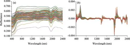
Fig.3 Reflectance curves of the original and preprocessed soil spectra.(a), original spectra; (b), spectra processed by Savitzky-Golay (SG) smoothing and first derivative (FD) processing.Note that the curves with different color represent the reflectance spectra of different soil samples.

3.3 Correlation analysis of the SOM content with original and preprocessed soil spectra

The correlation coefficient curves are derived by analyzing the correlation between the SOM content and preprocessed soil spectra (Fig.4).The correlation curve between the original spectra and the SOM content was relatively smooth, and only the 1810.0-1850.0 nm wavelengths passed significance testing at the 0.01 level, indicating that the sensitivity of the original spectra to the SOM content was low.Based on SG smoothing, the overall correlation of the FD-treated spectra was significantly improved, especially at 750.0-950.0 and 1220.0-2350.0 nm, with a maximum absolute correlation coefficient of 0.479 at 843.0 nm.There was a carbon-hydrogen (C-H) bond near this wavelength, which is directly related to the SOM content.Therefore, we selected 442 wavelengths that passed the significance test at the 0.01 level for subsequent comparative analysis and modelling predictions based on the results of the FD processing spectra.

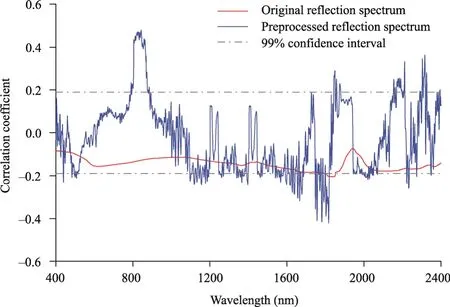
Fig.4 Correlation coefficient curves between the soil organic matter (SOM) content and preprocessed soil spectra

3.4 Characteristic wavelength optimization

3.4.1 CARS algorithm to extract feature variables

Figure 5 shows the variable selection process of the CARS algorithm.It can be seen that the number of retained wavelengths gradually decreased as the number of iterations increased, and the rate of decrease was from fast to slow (Fig.5a).The RMSECV showed a trend from large to small and then from small to large, and the RMSECV was the smallest (9.44) when the number of iterations was 26 (Fig.5b).This was because during the variable selection process from 1 to 26,the RMSECV decreased by continuously eliminating wavelengths that were less correlated with the SOM content and had little impact on the modelling results.After 26 iterations, the wavelengths with strong correlation with the SOM content started to be removed, resulting in an increase in the RMSECV.Figure 5c presents the stability trajectory of the wavelength variables.Each curve in the plot shows the trend of the stability of each variable with the number of iterations, and the optimal subset of variables with the smallest RMSECV is marked with an asterisk.Thus, the set of variables corresponding to the 26thsampling was the optimal subset of the SOM spectral variables, containing 31 spectral variables: 463.0, 468.0, 476.0, 790.0, 791.0, 792.0, 793.0, 794.0, 795.0, 803.0, 804.0,805.0, 806.0, 811.0, 812.0, 1338.0, 1347.0, 1348.0, 1349.0, 1350.0, 1816.0, 1817.0, 2177.0, 2178.0,2211.0, 2274.0, 2303.0, 2316.0, 2325.0, 2385.0, and 2386.0 nm.

Fig.5 Process of filtering variables by the competitive adaptive reweighted sampling (CARS) algorithm.(a),changing trend of the number of sampled variables with the increase of sampling runs; (b), changing trend of the root mean square error of cross-validation (RMSECV) with the increase of sampling runs; (c), trend regression coefficient paths with the increase of sampling runs.Note that the curves with different color represent the trend of the stability of each variable with the number of sampling runs, and the positions marked by vertical asterisks correspond to the optimal subset of variables that the RMSECV reached its minimum in the whole variable selection process.

3.4.2 SPA to extract feature variables

SPA was used to select the feature variables combined with the spectral data.The range of feature variable variation to be selected was set to from 1 to 10 (Fig.6), and the settings of the calibration set and prediction set samples were kept constant.Figure 6a shows the RMSE trend with the number of variables included in the model.During the change in the number of feature variables,the horizontal coordinate is the number of variables included in the model, and the vertical coordinate is the RMSE.As the number of variables included in the model increased, the minimum RMSE gradually decreased, reaching a minimum (9.47) when the number of variables included in the model reached 5.When the number of variables included in the model increased to close to 6, further increases introduced wavelength variables that were unrelated to the predicted values or variables with greater noise, and the RMSE then increased.Figure 6b shows the distribution of the feature variables on the first calibration object.The algorithm selected five optimal variables: 835.0, 1347.0, 1769.0, 1874.0, and 2177.0 nm.

Fig.6 Process of filtering variables by the successive projections algorithm (SPA).(a), variation in the root mean square error (RMSE) with the number of variables included in the model; (b), distribution of the feature variables on the first calibration object.

3.4.3 Boruta algorithm to select feature variables

When the Z score of the feature variable is larger than shadowMax, the feature is considered to be important.As seen in Figure 7, the maximum value of the shadowMax is 3.15, and there were 23 feature wavelengths with a Z score larger than the maximum value of the shadowMax, namely,488.0, 491.0, 806.0, 809.0, 822.0, 823.0, 824.0, 1221.0, 1243.0, 1466.0, 1447.0, 1560.0, 1561.0,1596.0, 1597.0, 1655.0, 1656.0, 1657.0, 1658.0, 1781.0, 1782.0, 2174.0, and 2175.0 nm.These 23 variables will be selected for modelling later.

3.5 Model construction and comparative analysis

Table 2 shows the results of the PLSR and RF models for the preselected and optimal variables.In the PLSR model, the prediction results based on the optimal wavelength were both better than those based on the preselected wavelength.Among them, the model prediction based on the CARS algorithm was the best, with an R2of 0.67 and an RPD of 2.12 in the model validation set,while the prediction accuracy of Boruta algorithm-PLSR (PLSR model based on the Boruta algorithm) on the validation set was second only to CARS-PLSR (PLSR model based on the CARS algorithm).Furthermore, compared to the PLSR model, the RF model based on preselected variables had an R2of 0.54 and an RPD of 1.64 for the validation set, showing a slight improvement in modelling results to roughly predict the sample.The best-performing model was Boruta algorithm-RF (RF model based on the Boruta algorithm), which had an R2of 0.78 and an RPD of 2.38 for the validation set.Next, the models built based on the feature wavelengths selected by CARS and SPA showed slightly worse performance results.However, the R2of the validation set was higher than that of the preselected variables, and the R2of the calibration set was closer to that of the validation set, which indicated that the stability of the built models was better.

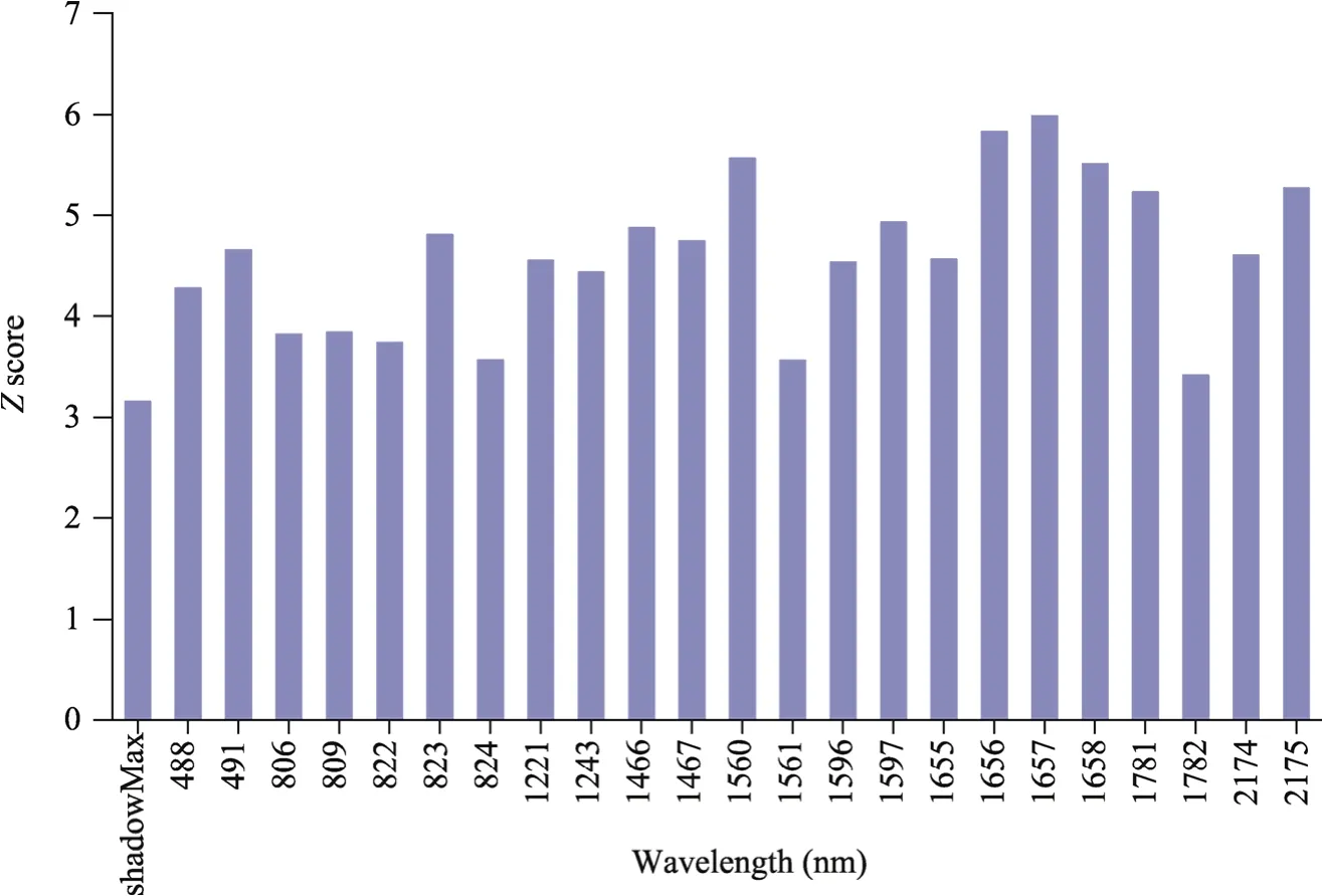
Fig.7 Importance score (Z score) of the different wavelengths identified by the Boruta algorithm

Table2 Comparison of the coefficient of determination (R2), root mean square error (RMSE), and residual prediction deviation (RPD) obtained from partial least squares regression (PLSR) and random forest (RF) models based on four wavelength selection methods

Figure 8 shows the distribution of the feature variables selected by the three variable selection methods.The number of variables selected by the three algorithms was significantly reduced compared with the preselected variables, and the least accounted for only 1.4% of the preselected variables.In addition, the optimal variables obtained by the three variable selection methods had similar distribution ranges.The variables were mainly distributed in the near-infrared spectral regions of 1200.0-1600.0, 1700.0-2000.0, and 2200.0-2400.0 nm.The fundamental and octave vibrational absorption of carbonyl (C=O), carbon-hydrogen (C-H), aluminium-hydroxy (Al-OH),and hydroxide (O-H) bonds is the main manifestations in the near-infrared spectral range (Jin et al., 2016), which is the main reason why vis-NIR spectra show special absorption peaks at approximately 1400.0, 1900.0, and 2200.0 nm.The absorption feature near 1400.0 nm is associated with hydroxyl (-OH) bonds, while the absorption wavelength near 1900.0 nm is the H2O spectrum dominated by interlayer water.The absorption wavelength near 2000.0 nm is a combination of -OH stretching vibrations with Al-OH and magnesium hydroxyl (Mg-OH)bending vibrations.However, the CARS and Boruta algorithms also selected a small number of SOM spectral features located in the 400.0-780.0 nm range of the visible spectrum.The result was consistent with the previous studies (Araújo et al., 2001; Nocita et al., 2014; Li et al., 2019).Therefore, this suggests that the preferred wavelength in this study is reasonable.

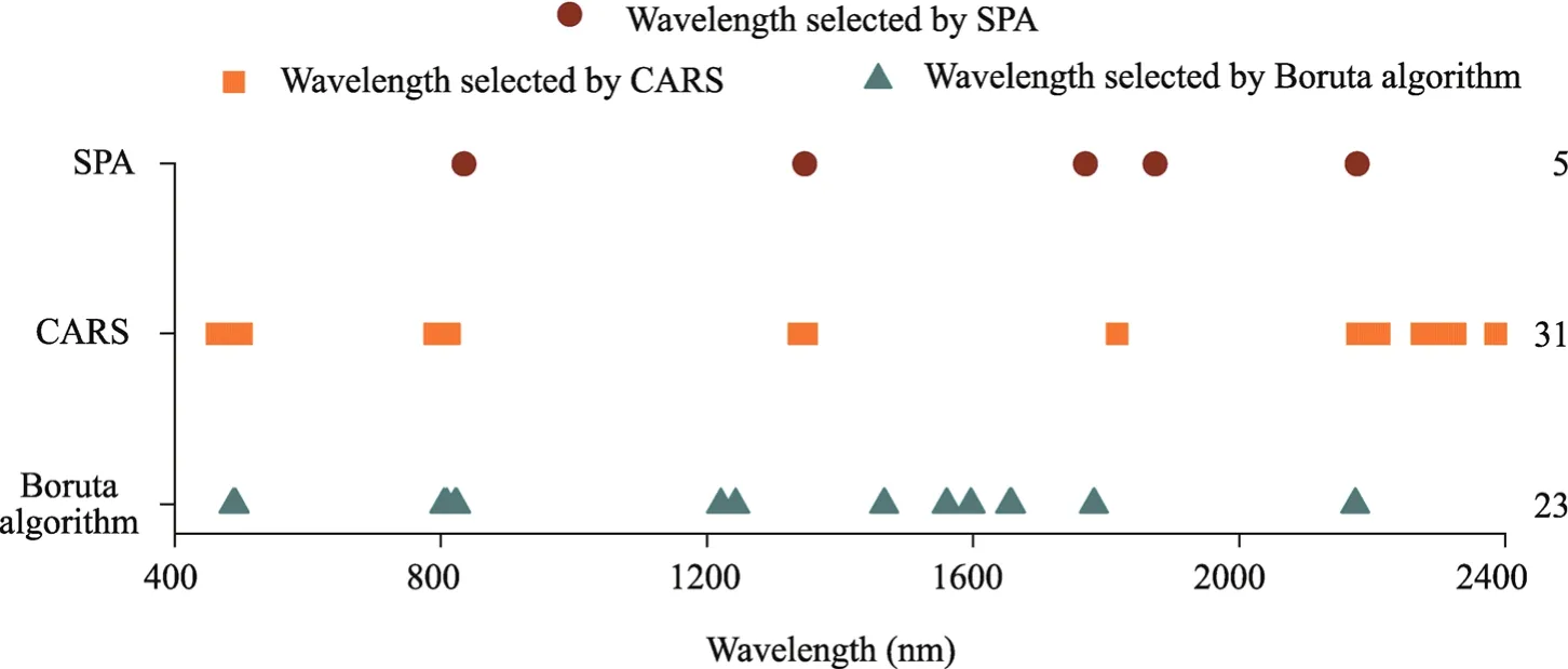
Fig.8 Distribution of feature variables selected by SPA, CARS, and Boruta algorithms.Note that the numbers on the right side of the figure represent the number of optimal variables selected by SPA, CARS, and Boruta algorithms.

Conventional selection methods for soil spectral variables are performed by Pearson correlation analysis.Correlation analysis only considers the simple linear pattern between the independent variable itself and the dependent variable, while the exploration of deeper nonlinear implied relationships and the elimination of the information redundancy phenomenon appear to be weak(Wang et al., 2019; Ge et al., 2021).Therefore, we suggest correlation analysis as a way to preselect variables.As shown in Table 2, the RPD of the two models was 1.24 and 1.64 for modelling by the significance wavelengths obtained from Pearson correlation analysis, indicating that the models could only achieve a relatively coarse estimation of soil information.This may be due to the presence of more redundant or irrelevant information among the selected variables,resulting in lower model accuracy (Nocita et al., 2014).However, the accuracy of the PLSR and RF models based on the three feature variable selection algorithms was further improved compared to the accuracy of the preselected wavelength model, and the R2of the validation set was improved by 25% on average, indicating the importance of optimal variable selection for the preselected wavelength.Compared to traditional linear regression models, machine learning algorithms have significant advantages (Araújo et al., 2014; Li et al., 2021).The poor performance of the PLSR model based on vis-NIR spectroscopy may be due to the indirect spectral response of SOM (Dharumarajan et al., 2022).The same variable selection methods used in the RF model in this study showed an increase in the R2and RPD of the test set, while the RMSR decreased.The results exhibited by the variable selection methods were not consistent for different modelling schemes.In the PLSR model, the CARS algorithm showed greater competitiveness, while the Boruta algorithm was second only to the CARS algorithm.Actually,the CARS algorithm is a linear method, while the PLSR model can better handle the linear information between spectra and SOM.The combination of PLSR and the CARS variable selection method can effectively improve the model accuracy, which is consistent with previous research results (Vohland et al., 2014).Among the nonlinear models, Boruta algorithm combined with the RF model had the best prediction accuracy among all the combined models, with R2improving by 0.10 and RMSE decreasing by 0.33 on average compared with other algorithms.This is because both Boruta algorithm and RF are nonlinear algorithms, and in addition, the Boruta algorithm is based on the RF classifier so that better prediction accuracy can be achieved(Hong et al., 2021).The poor performance of the SPA in both models may be because the SPA aims to eliminate the covariance between variables, while the projection is performed without including soil property information, and some of the spectral wavelengths with rich information are not selected, thus leading to a lower model performance (Araújo et al., 2001).In addition, as mentioned by Chen et al.(2001), for small datasets (fewer than 200 samples), cross-validation or repeated random splitting leads to more robust model evolution.

Although the spectral ranges selected by the three methods were approximately the same, the application of the different models showed very different results.Therefore, we suggest that when building the SOM content prediction model, a suitable modelling scheme should be implemented according to different variable selection strategies.This method was effective and fast in estimating the SOM content but lacked spatial expressiveness.Furthermore, the soil type was not taken into account in this study due to the different effects of different types of soil texture and composition on the spectral characteristics.Further research is needed on how to improve the spatial expressivity of the SOM content and on how to combine the SOM content prediction of different soil types to improve model accuracy.

The original spectra were preprocessed and preselected by Pearson correlation analysis, and then the CARS, SPA, and Boruta algorithms were used to select spectral feature wavelengths, and the PLSR and RF models were combined to construct SOM content prediction models for the selected feature variables.Among the three variable selection algorithms, the RF model based on the Boruta algorithm had the best accuracy in the prediction of the SOM content.The RF model based on the Boruta algorithm improved the R2to 0.78 and the RPD to 2.38, achieving accurate SOM content prediction.The regression model coupled with the variable selection algorithm greatly reduced the complexity of the model while ensuring the accuracy of the model and provided technical support for the rapid and nondestructive estimation of the SOM content of arid land using spectral analysis technology, with promising applications.

This study was supported by the Key Project of Natural Science Foundation of Xinjiang Uygur Autonomous Region, China (2021D01D06) and the National Natural Science Foundation of China (41961059).We thank anonymous reviewers for their insightful comments, which help improve the quality of this manuscript.